
Key takeaways
- 01
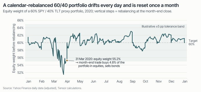
Rebalancing is a mechanical, calendar-anchored flow. A 60/40 proxy portfolio (SPY/TLT) that is reset every month-end had to trade a median 0.8% of its value at each month-end since 2002. In one month in ten the figure was 2.6% or more, and at the end of March 2020 it was 4.8%. In 84% of months the direction of that trade could be read from the stock–bond performance gap in the first 15 trading days.
- 02
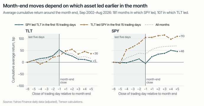
The footprint is visible in prices. Over the last five trading days of the month, TLT returned +42 bp on average, against +8 bp for an average five-day window. When equities led in the first half of the month, TLT gained 52 bp into month-end and gave back 48 bp in the first five days of the next month. When bonds led, SPY gained 105 bp into month-end.
- 03
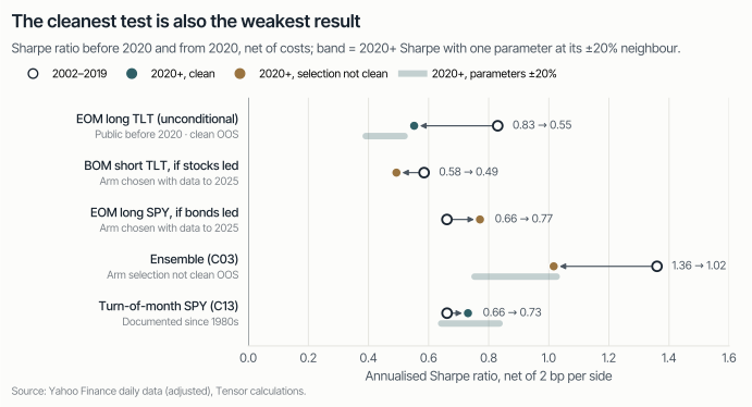
The cleanest test is also the weakest result. The unconditional month-end Treasury effect was in the public domain by November 2019. Since 2020 its Sharpe ratio has fallen from 0.83 to 0.55 (t = 1.4). A published three-arm variant shows 1.02 since 2020, but two of its three arms were chosen with data through June 2025. That figure is not out-of-sample evidence.
- 04
For allocators the useful lesson sits on the other side of the trade. Predictable calendar rebalancing costs money: one estimate puts it at about $16 billion a year for US investors. Tolerance bands, spread or randomised execution and careful use of the close usually matter more than harvesting the pattern.
Drift against a fixed target.
A portfolio with fixed target weights is always drifting. When equities outperform bonds, the equity weight rises; when they underperform, it falls. Rebalancing reverses the drift. The trade it requires is mechanical, not a view on either asset.
A useful rule of thumb: for a two-asset portfolio with target weight w, the rebalancing trade is approximately w(1 − w) times the return gap between the two assets. For a 60/40 mix that is 0.24 × the gap. A month in which equities beat bonds by five percentage points leaves the portfolio about 1.2% of its value away from target. The rebalancer has to sell that amount of equities and buy the same amount of bonds.
 Enlarge chart
Three design choices determine when the resulting flow reaches the market:
- Calendar vs. threshold. Harvey, Mazzoleni and Melone (2025) separate calendar rebalancing, which trades on a schedule, from threshold rebalancing, which trades once weights move a set distance from target. Calendar rebalancers make their timing public; only the size is uncertain. Threshold rebalancers make their trigger public; they trade after large moves, whenever those happen.
- Month vs. quarter. Less frequent rebalancing trades less often but lets drift accumulate. In our proxy, quarter-only rebalancing would have required a median trade of 1.7% of the portfolio each quarter-end, against 0.8% at each month-end under monthly rebalancing.
- Settlement and liquidity calendars. Etula et al. (2020) link month-end equity patterns to the institutional payment cycle. Under the three-day settlement convention in their sample, an institution that needs cash on the last day of the month “must sell securities at least 4 business days … before the month end”. US equity settlement moved to T+1 on 28 May 2024 (SEC, 2023). Timing conventions that shaped historical day-count patterns can therefore shift.
Bond indices add a second calendar. The Bloomberg (formerly Barclays) Treasury index is rebalanced on the final trading day of each month. On average three securities are added and three dropped at each rebalance (Hartley and Schwarz, 2019). Managers benchmarked to the index have a reason to adjust on the same day, whatever equities have done.
How large are the flows?
Precise, public, current flow estimates do not exist. Most figures in circulation are strategist estimates tied to specific months. We therefore rely on three kinds of evidence and label each one.
US retirement assets
Held in DB plans, DC plans and IRAs at year-end 2022 (Federal Reserve Financial Accounts, as cited by Harvey et al., 2025).
assumed rebalancing market
Harvey et al.’s working assumption for balanced capital that rebalances. It is an assumption, not a measured flow.
annual cost estimate
Back-of-the-envelope estimate by Harvey et al.: rebalancing costs above 8 bp a year on that market, or about $200 per US household.
annual cost, liquidity trading
Etula et al.’s estimate of what month-end liquidity-driven trading cost institutions each year over 1999–2013.
Market impact. Harvey et al. find that when stocks are overweight, “funds sell stocks and buy bonds, leading to a decrease in equity returns of 17 basis points over the next day.” This is the next-day effect of a one-standard-deviation move in their calendar signal. The pressure “revert[s] almost entirely within two weeks”, and calendar predictability “peaks in the last four days of the month”.
Strategist estimates. Sell-side desks publish quarter-end rebalancing estimates regularly. Bloomberg, for example, reported on 15 June 2023 that JPMorgan expected about $150 billion of equity selling from rebalancing. We could verify only the headline, not the method or the horizon, so we treat such numbers as indicative only.
A transparent rule of thumb. Our proxy converts drift into money without any assumption about who holds what. Each $1 trillion of monthly-rebalanced 60/40 capital implies about $8 billion of month-end trading in a median month and about $26 billion in one month in ten. Much of this nets internally or across funds, so the market-facing flow is smaller.
What the data show.
The mechanism makes a testable prediction. If balanced mandates sell the winner and buy the loser at month-end, then the stock–bond lead earlier in the month should tell us which asset receives buying pressure in the final days. The pressure should then partly reverse.
 Enlarge chart
| Window (compounded, mean per month) | All months | SPY led first half | TLT led first half |
|---|---|---|---|
| TLT, last five trading days | +42 bp (t 4.6) | +52 bp (t 4.5) | +26 bp (t 1.7) |
| TLT, first five days of next month | – | −48 bp (t −3.0) | +10 bp (t 0.5) |
| SPY, last five trading days | +35 bp (t 2.6) | −6 bp (t −0.4) | +105 bp (t 3.7) |
| Reference: any five-day window | TLT +8 bp · SPY +25 bp | ||
| Number of months | 288 | 181 | 107 |
Scroll horizontally to see all columns.
Three observations stand out.
- Treasuries rally into month-end regardless. The unconditional TLT effect is present in both regimes. It fits the index-calendar explanation of Hartley and Schwarz (2019): “Average returns are positive and highly significant in the last few days of the month, and are not significantly different from zero at other times.” They also find that “life insurers are large net buyers of Treasury securities on benchmark index rebalancing dates.”
- The conditional pattern matches rebalancing. When equities led, bonds gained into month-end and then lost it. When bonds led, equities gained into month-end. This is the direction the drift arithmetic predicts. It is also consistent with the turn-of-month equity literature. McConnell and Xu (2008) find that over 1926–2005, “investors received no reward for bearing market risk except at turns of the month”.
- Quarter-ends are not larger in this sample. Quarter-end months should carry more drift, yet TLT’s last-five-day return averaged +31 bp (t 2.0) in quarter-end months against +48 bp (t 4.2) in the others. The pattern for SPY was similar. The most anticipated dates do not show the strongest effect. That is consistent with front-running, or with other quarter-end balance-sheet flows offsetting the rebalancing flow, but this data cannot tell the two apart.
What survives costs, publication and a clean out-of-sample test.
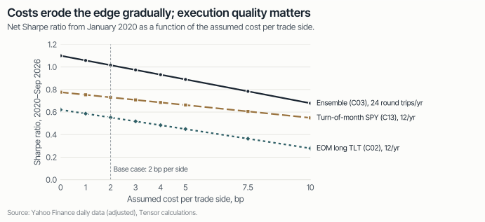
A persistent pattern in averages is not the same as a strategy that survives implementation. We test three published rules exactly as posted, with no re-optimisation. All are calendar rules executed at the close with 2 bp per side:
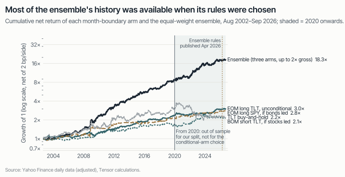
- EOM long TLT: long TLT over the last five trading days of every month.
- Month-boundary ensemble: EOM long TLT, plus EOM long SPY when bonds led the first 15 days, plus short TLT over the first five days of the next month when stocks led (Beyond Passive, 2026, with SPY in place of VTI).
- Turn-of-month SPY: long SPY from the fifth-last trading day to the third trading day of the new month.
 Enlarge chart
The chart’s apparent message, a smooth ensemble line and every calendar year from 2003 to 2025 positive, is exactly why we are careful with it. The rules were published in April 2026. Their author chose the conditional arms from five candidate sleeves, using “273 months through June 2025”. Our 2020 split therefore protects nothing for those two arms: the data after 2020 was in the author’s selection sample.
The only component with a clean out-of-sample period is the unconditional month-end Treasury effect. It was documented in a public working paper in November 2019 (Hartley and Schwarz), so our 2020 split falls after publication.
| Net Sharpe ratio | Full sample | 2002–2019 | 2020–2026 | t-stat 2020+ | 2020+ at 2× costs | 2020+ gross | 2020+ with parameters ±20% | Time invested |
|---|---|---|---|---|---|---|---|---|
| EOM long TLT (clean OOS) | 0.75 | 0.83 | 0.55 | 1.4 | 0.48 | 0.62 | 0.39–0.52 | 24% |
| Month-boundary ensemble | 1.25 | 1.36 | 1.02* | 2.6 | 0.93 | 1.10 | 0.75–1.03 | 39% |
| Turn-of-month SPY | 0.68 | 0.66 | 0.73 | 1.9 | 0.69 | 0.78 | 0.64–0.84 | 33% |
| TLT buy-and-hold | 0.31 | 0.55 | −0.19 | 100% | ||||
| SPY buy-and-hold | 0.65 | 0.60 | 0.82 | 100% |
Scroll horizontally to see all columns.
* Not out-of-sample for the choice of the conditional arms. Samples begin 31 July 2002 (TLT rules) and 1 February 1993 (SPY rules). Cash earns 0% for strategy and buy-and-hold alike.
 Enlarge chart
What we read from the numbers:
- The clean effect weakened but did not disappear. The unconditional EOM TLT rule fell from 0.83 to 0.55. Its annualised mean dropped from 5.1% to 3.9% and its volatility rose from 6.2% to 7.1%. It stayed positive through a period in which TLT itself had a negative Sharpe ratio. Our base parameter was the best of the three neighbours after 2020, a mild warning in itself. A Sharpe ratio of 0.55 needs roughly 13 years to reach t = 2, and we have fewer than seven.
- Selection is the binding risk, not costs. For liquid ETFs at 2 bp per side, costs take about 0.5% a year from the TLT rule. Its break-even cost since 2020 is roughly 18 bp per side. Doubling costs moves the ensemble’s 2020+ Sharpe from 1.02 to 0.93. The larger uncertainty is how much of the 1.02 is a genuine forward result rather than a record of choices made with hindsight. Only live data after April 2026 can answer that, and at a Sharpe ratio near 1 it takes about four years to reach t = 2.
- The turn-of-month equity effect is real but not a free lunch. It matched SPY’s full-sample Sharpe ratio while invested a third of the time. Since 2020 it has trailed buy-and-hold (0.73 against 0.82).
- Losing streaks are normal. The unconditional TLT rule lost money in 2004, 2006, 2017, 2022 and 2023. A practitioner who documented the effect publicly stopped trading it during the 2023–2024 flat period and missed the 2025 recovery, as Beyond Passive (2026) recounts.
 Enlarge chart
What this means for allocators.
For most investors the useful side of this research is not harvesting the flow but paying less for their own. A calendar rebalancer publishes its timing to everyone who can read a calendar.
Know your footprint
Measure implementation shortfall on rebalancing trades separately, by day relative to month-end and against a mid-month benchmark.
Prefer bands to dates
Vanguard (Jaconetti et al., 2010) find “no optimal frequency or threshold” and suggest that “annual or semiannual monitoring, with rebalancing at 5% thresholds” balances risk control against cost.
Break the schedule
Harvey et al. show that “simple randomization in rebalancing schedules … largely eliminates these costs”. Spreading trades over several days has a similar aim.
Use the flows you already have
Directing contributions, redemptions and coupon income towards the underweight asset reduces the size of the discretionary trade.
Treat the close with care
Month-end closing auctions concentrate predictable demand. Check closing-auction imbalances, and consider futures overlays for the drift instead of cash-market trades.
Do not mistake the pattern for alpha
A published calendar pattern with a Sharpe ratio around 0.5–1.0 is crowded by construction. It can take years to tell decay from bad luck, and hindsight selection flatters every backtest.
The flows are real and the calendar is public. That is exactly why the edge should be expected to shrink, and why the cheaper win for most portfolios is to stop being predictable.
Methodology
- Data. Yahoo Finance daily OHLC, adjusted for dividends and splits (auto-adjusted), downloaded 23 September 2026. SPY from 29 January 1993, TLT from 30 July 2002, both to 21 September 2026. The data are not point-in-time curated.
- Rules. Taken exactly as published; nothing was re-optimised for this note. The Beyond Passive ensemble uses SPY instead of VTI and a weight of 1 per arm. The first-half lead is measured over the first 15 trading days, or up to the day before the month-end window in short months, so there is no look-ahead.
- Execution. Pure calendar rules are known in advance and executed at the close (market-on-close). No borrowing cost is charged for the TLT short, which is active about 15% of the time.
- Costs and metrics. 2 bp per side on every change in position, plus 0×, 2× and a 0–10 bp grid. Sharpe = mean ÷ standard deviation of daily returns × √252, with 0% cash for strategies and buy-and-hold alike.
- Samples. In-sample to 31 December 2019; out-of-sample from 1 January 2020. For a single parameter at a time, the ±20% neighbours are tested.
- Proxy. The 60/40 proxy uses SPY and TLT total-return prices, rebalanced at the last close of each month.
- Reproducibility. Every figure is recomputed by
compute.pyandcharts.pyfrom a byte-identical snapshot of the research harness. All Sharpe ratios reproduce the original run to 1e-9. The source run tested 17 published rule variants, and 11 of them clear a Bonferroni-style full-sample hurdle of |t| ≈ 3. Several of those decay after 2020, so full-sample t-statistics say little on their own; this note therefore puts post-2020 and post-publication behaviour first. - Final month. The data end on 21 September 2026, and the source run treats that incomplete month as if it had ended then. Excluding it lowers the 2020+ Sharpe ratios slightly: EOM TLT to 0.53, the ensemble to 1.01 and turn-of-month SPY to 0.69. The event study excludes it.